Remember when Daylight Saving Time happened to us again? You know, that day that causes us all to grumble loudly about the ridiculousness of our biannual clock adjustment and loss of sleep?
In this post, I engage in some self-care data visualization to explore day light hours in cities across the world and the United States, inspired by an awesome night hours series by Krisztina Szucs.
Are we saving daylight in Atlanta, GA?
As a parent, I loathe daylight saving time. Nothing reveals the shared delusion of time like trying to explain to your children why we moved the clock forward an hour when it means they’ll suddenly need to go to bed while it’s light out or wake up and get ready for school while it’s dark.
So in this spirit, I started to wonder: what kind of returns are we getting on our daylight saving? Except, rather than try to directly answer that question — since that’s way too hard — I chose to visualize day light hours to see how they align with the modern work day.
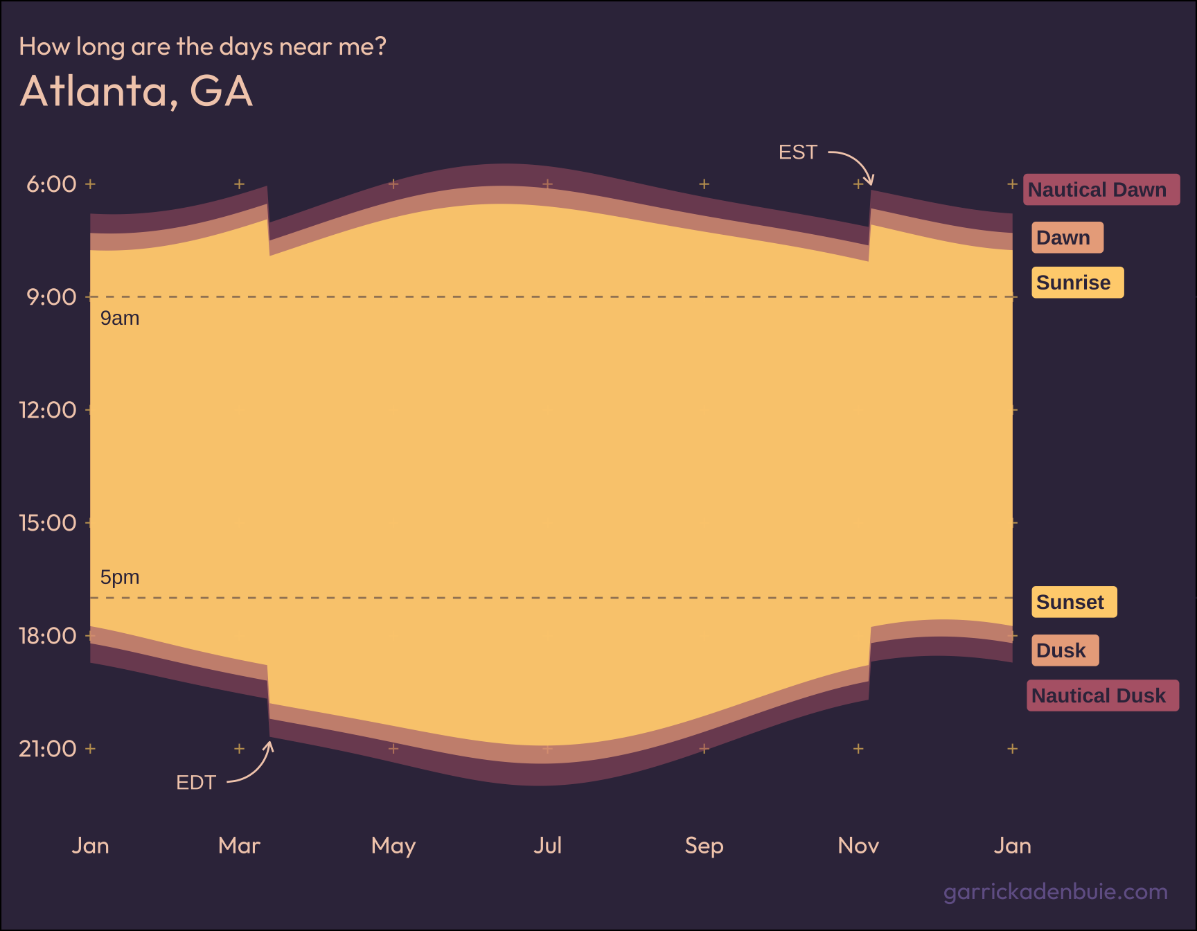
The plot below shows the yearly day light schedule for 2022 in Atlanta, GA where I live. We’ll also take a look at the day light schedule in other cities around the world or across the United States. At the end of this post, I’ll share the code I used to make the plot below.
| Date | Sunrise | Sunset | Daylight | Non-Work | |
|---|---|---|---|---|---|
| Shortest Day | Dec 21 | 7:41 am | 5:38 pm | 9h 56m | 1h 56m |
| Longest Day | Jun 21 | 6:32 am | 8:54 pm | 14h 21m | 6h 21m |
It’s pretty clear from this visualization that in Atlanta, GA, which is very much on the western edge of the U.S. Eastern time zone, year-round standard time is a decent way to live life. What about other cities in the world?
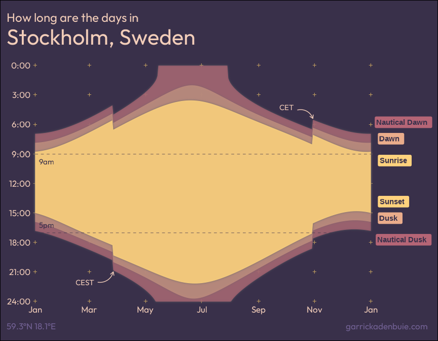
Around the World
Across the US
It seems that every year we talk about finally doing something about daylight saving time, but this year the U.S. Senate actually went so far as to pass a bill to make Daylight Saving Time permanent. In a suprising-to-no-one twist, the bill is stalled in the House, where representatives are arguing over which of standard or daylight saving time should be permanent.
Would you prefer standard time or daylight saving time? If you’re not sure, check out the Daylight Saving Time Gripe Assistant Tool by Andy Woodruff on Observable.
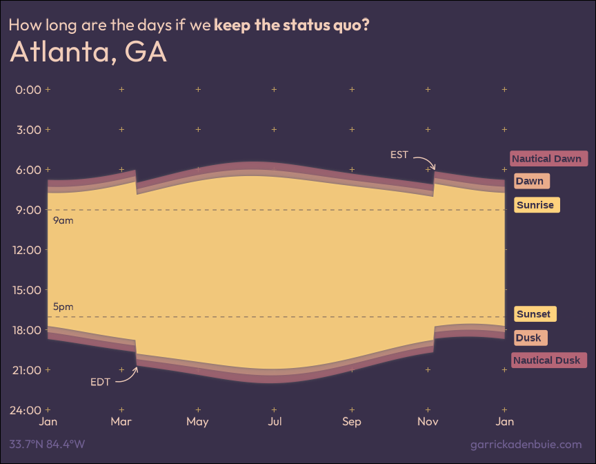
I thought it’d be interesting to visualize day light hours for U.S. cities. You can use the dropdown below to choose your city or the nearest city with more than 100,000 residents (or just pick a random city!). Then, toggle between Standard or DST to see how either proposal would affect you. Or choose Both to see what will happen in the unimaginable case that the U.S. Congress doesn’t actually make DST permanent.

Inspiration
The layout for this vizualization was heavily inspired by a series by Kristina Szucs that I discovered via r/dataisbeautiful. I loved the aesthetic of Kristina’s plot and the subtle gradients and shadows of the daylight/twilight hour regions. Her attention to little details such a the sunrise and sunset icon labels and the stars in the night region are just fantastic.
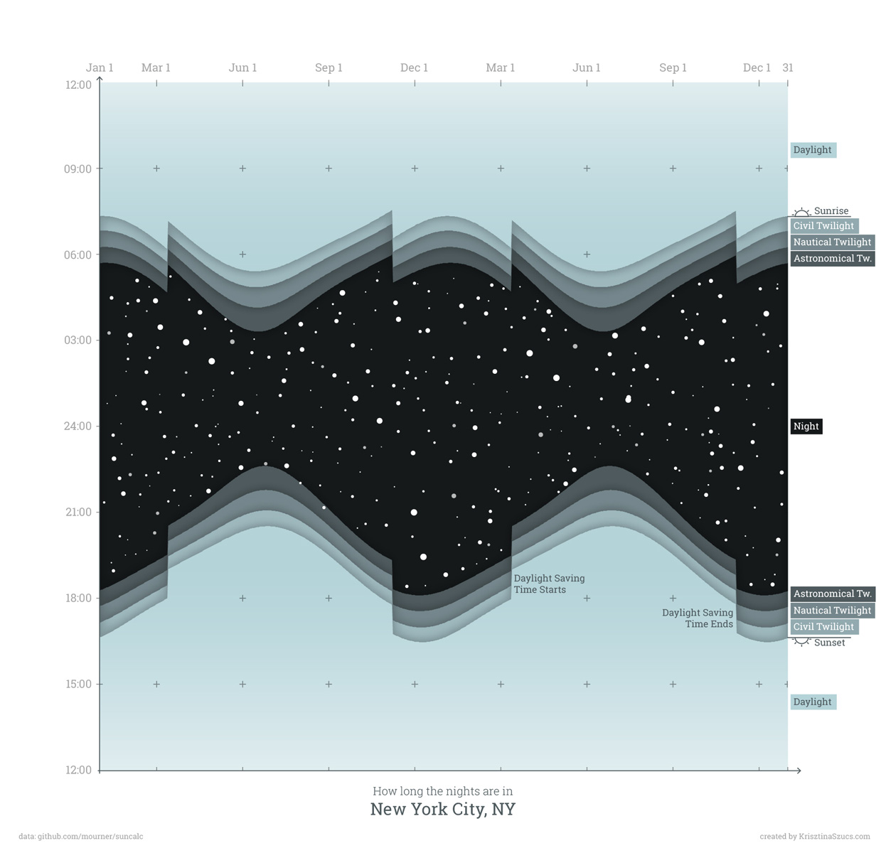 How long are the nights in New York City? by Krisztina Szucs
In my version I wanted to draw on a similar structure and style to visualize daylight rather than sunset hours. I also wanted to see how far I could go with my plot without leaving the comfort of ggplot2, so I stopped short of adding the sunrise and sunset icons. (I suppose anything is possible in ggplot2 but IMHO this is a reasonable line to draw.)
Where are you?
To get accurate sunrise and sunset time data, we first need to figure out where in the world we are. Fortunately, the ipapi package makes it easy to grab key geolocation data from your IP address, like latitude, longitude and time zone. (I’m adding a little fuzz just to make ipapi a little less accurate.)
location <- as.list(ipapi::geolocate(NA, .progress = FALSE))

# find a location nearby but not my actual house, lol
location$lat <- location$lat + runif(1, min = -0.5, max = 0.5)
location$lon <- location$lon + runif(1, min = -0.5, max = 0.5)location[c("lat", "lon", "timezone")]
## $lat
## [1] 33.34846
##
## $lon
## [1] -85.17511
##
## $timezone
## [1] "America/New_York"Sunrise and Sunset Times
Next, we take our latitude and longitude to suncalc, an R package port of suncalc.js. We ask getSunlightTimes() for the dawn and dusk related times for every day in 2022.
sun_times <-
  suncalc::getSunlightTimes(
    date = seq(
      as.Date("2022-01-01"),
      as.Date("2023-01-01"),
      by = "day"
    ),
    lat = location$lat,
    lon = location$lon,
    tz = location$timezone,
    keep = c("dawn", "nauticalDawn", "dusk", "nauticalDusk", "sunrise", "sunset")
  )

head(sun_times)
##         date      lat       lon                dawn        nauticalDawn
## 1 2022-01-01 33.34846 -85.17511 2022-01-01 07:18:23 2022-01-01 06:47:27
## 2 2022-01-02 33.34846 -85.17511 2022-01-02 07:18:35 2022-01-02 06:47:41
## 3 2022-01-03 33.34846 -85.17511 2022-01-03 07:18:45 2022-01-03 06:47:53
## 4 2022-01-04 33.34846 -85.17511 2022-01-04 07:18:54 2022-01-04 06:48:03
## 5 2022-01-05 33.34846 -85.17511 2022-01-05 07:19:02 2022-01-05 06:48:12
##                  dusk        nauticalDusk             sunrise
## 1 2022-01-01 18:12:28 2022-01-01 18:43:24 2022-01-01 07:45:47
## 2 2022-01-02 18:13:11 2022-01-02 18:44:05 2022-01-02 07:45:57
## 3 2022-01-03 18:13:54 2022-01-03 18:44:47 2022-01-03 07:46:06
## 4 2022-01-04 18:14:39 2022-01-04 18:45:30 2022-01-04 07:46:14
## 5 2022-01-05 18:15:25 2022-01-05 18:46:14 2022-01-05 07:46:19
##                sunset
## 1 2022-01-01 17:45:04
## 2 2022-01-02 17:45:48
## 3 2022-01-03 17:46:33
## 4 2022-01-04 17:47:20
## 5 2022-01-05 17:48:07
##  [ reached 'max' / getOption("max.print") -- omitted 1 rows ]
If you’re curious about the difference between (civil) dawn, nautical dawn and sunrise, take a stroll through Twilight on Wikipedia.
Tidy Sun Times
As cool as it is to so easily get to the point of having this data in hand, we need to do a little bit of tidying up to get it ready for ggplot2. In particular, we need to consolidate all of the timestamps into one column that we can index by date and event (such as dawn, nautical dawn, etc.). I used pivot_longer() to move the column labels for dawn through sunset into an event column with the corresponding values from each row in an adjacent time column.
library(tidyverse)

tidy_sun_times <-
  sun_times %>%
  select(-lat, -lon) %>%
  pivot_longer(-date, names_to = "event", values_to = "time") %>%
  mutate(
    tz = strftime(time, "%Z"),
    time = hms::as_hms(time)
  )

tidy_sun_times
## # A tibble: 2,196 × 4
##    date       event        time     tz
##    <date>     <chr>        <time>   <chr>
##  1 2022-01-01 dawn         07:18:23 EST
##  2 2022-01-01 nauticalDawn 06:47:27 EST
##  3 2022-01-01 dusk         18:12:28 EST
##  4 2022-01-01 nauticalDusk 18:43:24 EST
##  5 2022-01-01 sunrise      07:45:47 EST
##  6 2022-01-01 sunset       17:45:04 EST
##  7 2022-01-02 dawn         07:18:35 EST
##  8 2022-01-02 nauticalDawn 06:47:41 EST
##  9 2022-01-02 dusk         18:13:11 EST
## 10 2022-01-02 nauticalDusk 18:44:05 EST
## # … with 2,186 more rows
There’s also a small trick here to use strftime() to extract the short timezone label %Z, e.g. EST or EDT, for each day, which I’ll use later when calling out the time changes. And finally, I used hms::as_hms() to extract the time of day component from each sun event timestamp. The neat thing about the hms class is that while it prints in a readable hours, minutes, seconds format, we can also treat it as an integer number of seconds from midnight. We’ll use this property in just a bit when working on the plot’s axis labels.
First Looks
Now that we have tidy data ready for ggplot2, let’s plot it! This plot won’t look amazing, but it will help us get a sense of the data we have to work with.
ggplot(tidy_sun_times) +
  aes(x = date, y = time, color = event) +
  geom_line()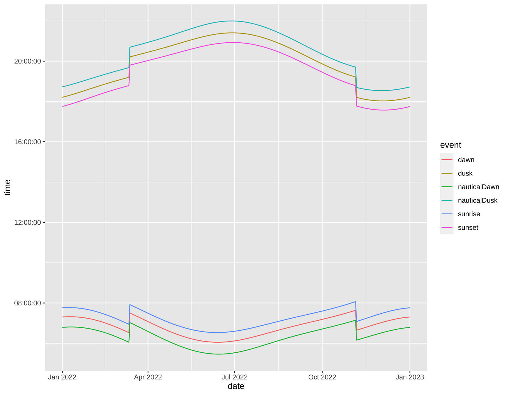
Paired Daily Events
The plot above reveals our next challenge: I used geom_line() to plot the time of each event as a line, but I want to be able to fill in the region between each pair of events:
- sunrise and sunset
- dawn and dusk
- nautical dawn and nautical dusk.
We can use geom_ribbon() to acheive this look, but it requires a little more transformation. We need the sunrise time in one column called starts and a second column with the sunset time in ends. Then we can map these new columns to the ymin and ymax aesthetics, letting geom_ribbon() fill in space between them.
The plan of action is to create a new column that I’ll call period where we’ll choose which of these two new columns a timestamp will be moved to. We’ll identify each pair using the morning event label.
Because we need pivot_longer() to create two new columns, starts and ends, from our single period column, we’ll first split the table into a list of two tables, one for each period, and then pivot the timestamp column into a new column. Because we’re operating on a list, we’ll use purrr::map() to coordinate this action. Then we can merge the two tables back together with left_join(), using purrr::reduce() to apply that action to the list of pivoted tables.
After that, we’re back in single-table land, and can use mutate() and select() to tweak the final table output to make sure that the morning events are ordered correctly: nautical dawn, then dawn, then sunrise.
tidier_sun_times <-
  tidy_sun_times %>%
  mutate(
    period = case_when(
      str_detect(event, "[dD]awn|sunrise") ~ "starts",
      str_detect(event, "[dD]usk|sunset") ~ "ends"
    ),
    pair = recode(
      event,
      nauticalDusk = "nauticalDawn",
      sunset = "sunrise",
      dusk = "dawn"
    )
  ) %>%
  group_split(period) %>%
  map(pivot_wider, names_from = "period", values_from = "time") %>%
  reduce(
    left_join,
    by = c("date", "tz", "pair"),
    suffix = c("_ends", "_starts")
  ) %>%
  mutate(
    pair = factor(pair, c("nauticalDawn", "dawn", "sunrise"))
  ) %>%
  select(date, tz, pair, contains("starts"), contains("ends"))

tidier_sun_times
## # A tibble: 1,098 × 7
##    date       tz    pair         event_starts starts   event_ends   ends
##    <date>     <chr> <fct>        <chr>        <time>   <chr>        <time>
##  1 2022-01-01 EST   dawn         dawn         07:18:23 dusk         18:12:28
##  2 2022-01-01 EST   nauticalDawn nauticalDawn 06:47:27 nauticalDusk 18:43:24
##  3 2022-01-01 EST   sunrise      sunrise      07:45:47 sunset       17:45:04
##  4 2022-01-02 EST   dawn         dawn         07:18:35 dusk         18:13:11
##  5 2022-01-02 EST   nauticalDawn nauticalDawn 06:47:41 nauticalDusk 18:44:05
##  6 2022-01-02 EST   sunrise      sunrise      07:45:57 sunset       17:45:48
##  7 2022-01-03 EST   dawn         dawn         07:18:45 dusk         18:13:54
##  8 2022-01-03 EST   nauticalDawn nauticalDawn 06:47:53 nauticalDusk 18:44:47
##  9 2022-01-03 EST   sunrise      sunrise      07:46:06 sunset       17:46:33
## 10 2022-01-04 EST   dawn         dawn         07:18:54 dusk         18:14:39
## # … with 1,088 more rows
Another plot
Now we’re ready to try out our even tidier data set! Okay, it’s actually less tidy, but more ready for plotting. We’ll swap out geom_line() for geom_ribbon(), and map starts to ymin and ends to ymax, filling in each region by pair.
ggplot(tidier_sun_times) +
  aes(date, ymin = starts, ymax = ends, fill = pair) +
  geom_ribbon()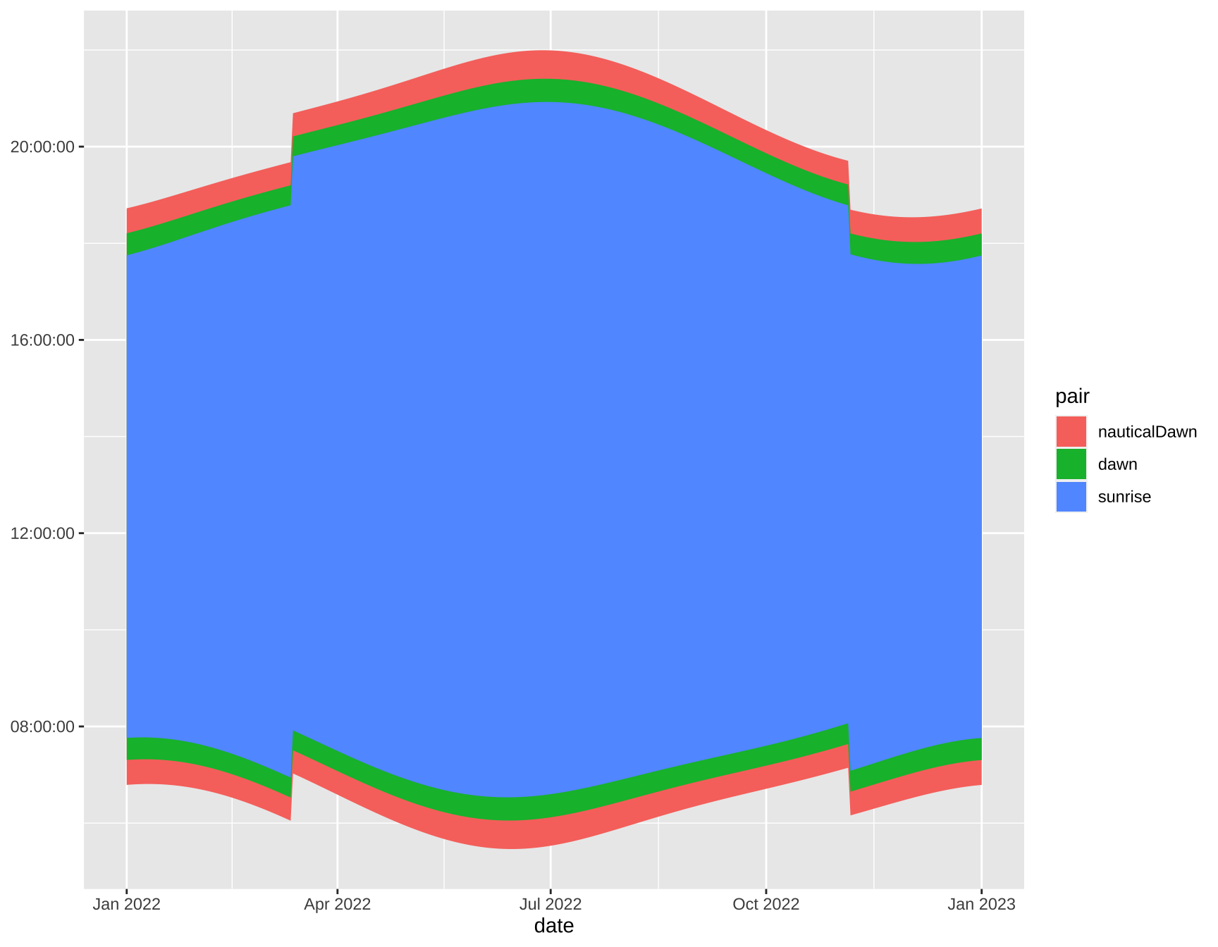
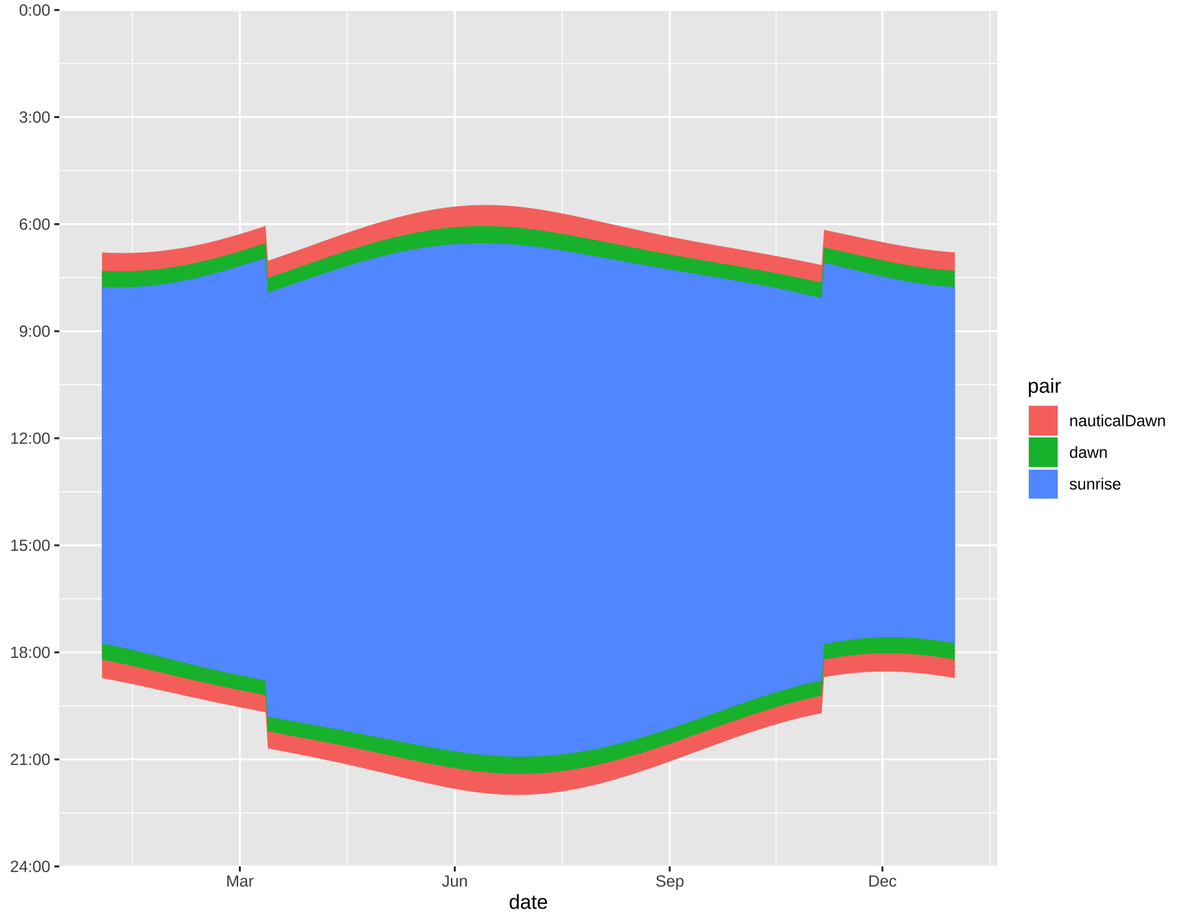
It looks terrible, but it’s more or less what we want to see. The y-axis is a little confusing though because it reads from night at the top to day at the bottom. The trick is to recall that we used hms::as_hms() to turn the time of day into an integer number of seconds from midnight. So we can reverse the y-axis with scale_y_reverse() and then provide our own labels.
ggplot(tidier_sun_times) +
  aes(date, ymin = starts, ymax = ends, fill = pair) +
  geom_ribbon() +
  scale_y_reverse(
    limits = c(24*60^2, 0),
    breaks = seq(0, 24*60^2, by = 3 * 60^2),
    label = paste0(seq(0, 24, by = 3), ":00"),
    expand = expansion()
  ) +
  scale_x_date(
    breaks = "3 months",
    date_labels = "%b"
  )
Make it pretty
Great! Now it’s time to draw the rest of the owl! Which means I’m now going to include roughly 150 lines of code that take the rough sketch above and make it a pretty ggplot.
Of course I should mention that what you’ll find below isn’t even the full story of the plots you see in this post. It turned out to be an intermediate sketch of the code that I actually used to create the plots. It also turns out that I’m pretty good at writing code that creates more problems that I need to solve with more code.
A few preliminaries: I’ll use the Outfit font from Google Fonts with the help of the sysfonts package.
sysfonts::font_add_google("Outfit")We’ll need a grid for the x- and y-axis that will be used in a few places, so I’ll create them up front. We end up with a vector of dates from January 1, 2022 to January 1, 2023 by 2 months for the x-axis and a vector of times from midnight to midnight by 3 hours for the y-axis.
x_breaks <- seq(
  from = as.Date("2022-01-01"),
  to = as.Date("2023-01-01"),
  by = "2 months"
)
y_breaks <- seq(0, 24*60^2, by = 3 * 60^2)
Finally, there are a couple of colors I used in more than one place for the foreground and background colors. There are a few other colors that I should have pulled into variables for clarity, but I’ve decided that it’s not worth the effort to think up variable names for them.
color_text <- "#F2CDB9"
color_bg <- "#39304a"
Finally, as promised, the 150ish lines of ggplot2 code. Enjoy!
ggplot(tidier_sun_times) +
  # The x-axis is always the day of the year
  aes(x = date) +
  # Behind everything we add a grid of `+` characters
  # in place of grid lines, to give a starry feel
  geom_text(
    # the data for this layer is our grid of x and y breaks
    data = cross_df(
      list(date = x_breaks, time = y_breaks, label = "+")
    ) %>%
      mutate(across(date, as.Date, origin = "1970-01-01")),
    aes(label = label, y = time),
    color = "#C29F5F"
  ) +
  # Here you'll recognize the outlines of our original plot sketch
  geom_ribbon(
    aes(ymin = starts, ymax = ends, fill = pair, alpha = pair),
    show.legend = FALSE
  ) +
  # Add dotted horizontal lines at 9am and 5pm
  geom_hline(
    yintercept = c(9, 17) * 60^2,
    color = color_bg,
    alpha = 0.5,
    linetype = 2
  ) +
  # And a little text to indicate the meaning of those lines
  annotate(
    geom = "text",
    x = min(tidier_sun_times$date),
    y = c(9, 17) * 60^2,
    label = c("9am", "5pm"),
    color = color_bg,
    hjust = -0.25,
    vjust = c(2, -1)
  ) +
  # If the timezone changes, it'll be due to daylight saving time
  # so we'll add a little text to highlight that change
  geom_text(
    # This combines my favorite magrittr pipe trick:
    #   `. %>%` creates a function with a single argument
    # with my favorite ggplot2 geom trik:
    #   `data` takes a function with a single argument that
    #   can be used to filter the global dataset to a smaller subset
    # The net result here is that we take the global data
    # and filter down to the two places where the timezone changes
    data = . %>%
      filter(tz != coalesce(lag(tz), first(tz))) %>%
      slice_head(n = 1),
    aes(y = ends, label = tz),
    hjust = 1,
    vjust = 1,
    nudge_x = -21,
    nudge_y = -60^2 * 1.5,
    lineheight = 0.8,
    color = color_text
  ) +
  # These add two little arrows to point from the timezone text
  # to the notch in the plot where the timezone change happens
  geom_curve(
    # Here's the `data = . %>%` trick again
    data = . %>%
      filter(pair == "nauticalDawn") %>%
      filter(tz != coalesce(lag(tz), first(tz))) %>%
      slice_head(n = 1),
    # This next bit took much fiddling.
    aes(
      x = date - 17,
      xend = date,
      y = ends - (-60^2 * 1.2),
      yend = ends + 500
    ),
    # If you like it put an arrow on it
    arrow = arrow(length = unit(0.08, "inch")),
    size = 0.5,
    color = color_text,
    curvature = 0.4
  ) +
  # The next two geoms highlight the second timezone change
  # and are copies of the previous two layers but use
  # `slice_tail()` instead of `slice_head()`.
  geom_text(
    data = . %>%
      filter(tz != coalesce(lag(tz), first(tz))) %>%
      slice_tail(n = 1),
    aes(y = starts, label = tz),
    hjust = 1,
    nudge_x = -21,
    nudge_y = 60^2 * 1.5,
    lineheight = 0.8,
    color = color_text
  ) +
  geom_curve(
    data = . %>%
      filter(pair == "nauticalDawn") %>%
      filter(tz != coalesce(lag(tz), first(tz))) %>%
      slice_tail(n = 1),
    aes(
      x = date - 17,
      xend = date,
      y = starts - 60^2,
      yend = starts - 500
    ),
    arrow = arrow(length = unit(0.08, "inch")),
    size = 0.5,
    color = color_text,
    curvature = -0.4
  ) +
  # Finally, we add a little annotation in the left edge of the plot
  # to serve as a legend for each layer and call out dawn, dusk,
  # sunrise and sunset, etc. Here I used the `ggrepel` package to
  # make sure the labels don't overlap, and in hopes that I wouldn't
  # need to fiddle too much with positioning. Fiddling was required
  # but I think the end result looks pretty good.
  ggrepel::geom_label_repel(
    data = . %>% filter(date == max(date)) %>%
      pivot_longer(contains("event")) %>%
      mutate(
        date = date + 12,
        time = if_else(value == pair, starts, ends),
        value = snakecase::to_title_case(value)
      ),
    aes(y = time, fill = pair, label = value),
    color = color_bg,
    fontface = "bold",
    show.legend = FALSE,
    # Most of the next few lines are designed to keep the
    # labels on the right side of the plot as close to the
    # layers they're supposed to annotate as possible.
    direction = "y",
    min.segment.length = 20,
    hjust = 0,
    label.size = 0,
    label.padding = 0.33,
    box.padding = 0.25,
    xlim = c(as.Date("2023-01-07"), NA)
  ) +
  # Next up, deal with our scales.
  # First up colors are the colors for the ribbon fill.
  scale_fill_manual(
    values = c(
      nauticalDawn = "#b56576",
      dawn = "#eaac8b",
      sunrise = "#ffd27d"
    )
  ) +
  # Then add a little opacity, even though ggplot will warn us
  # that using opacity with a discrete variable isn't a good idea.
  # (I think it's a fine idea, thank you very much.)
  scale_alpha_discrete(range = c(0.5, 0.9)) +
  # Here are the x- and y-axis scales from our original sketch
  scale_x_date(
    breaks = x_breaks,
    date_labels = "%b",
    limits = c(
      as.Date("2022-01-01"),
      as.Date("2023-03-15")
    ),
    expand = expansion()
  ) +
  scale_y_reverse(
    limits = c(
      max(tidier_sun_times$ends + 60^2),
      min(tidier_sun_times$starts - 60^2)
    ),
    breaks = y_breaks,
    labels = paste0(seq(0, 24, by = 3), ":00"),
    expand = expansion()
  ) +
  # Labels, obvs.
  labs(
    x = NULL,
    y = NULL,
    title = "How long are the days near me?",
    subtitle = "Atlanta, GA",
    caption = "garrickadenbuie.com"
  ) +
  # Make sure the sunrise/sunset labels aren't clipped by the plot area
  coord_cartesian(clip = "off") +
  # Finally, make it pretty. We'll start with a minimal base theme
  theme_minimal(base_family = "Outfit", base_size = 16) +
  # And then tweak a bunch of little things...
  theme(
    plot.title = element_text(
      color = color_text,
      hjust = 0,
      size = 14
    ),
    plot.subtitle = element_text(
      color = color_text,
      hjust = 0,
      size = 24,
      margin = margin(b = 6)
    ),
    plot.title.position = "plot",
    plot.background = element_rect(fill = color_bg),
    plot.margin = margin(20, 0, 20, 10),
    panel.grid = element_blank(),
    axis.text = element_text(color = color_text),
    axis.title = element_text(color = color_text),
    plot.caption = element_text(
      color = "#726194",
      hjust = 0.97,
      vjust = -1
    ),
    plot.caption.position = "plot"
  )