library(tidyverse)
library(gganimate)
library(babynames)
Earlier this week, a tweet from Kieran Healy caught my attention with a neat animation of the popularity of the final letters of baby names.
Using gganimate to visualize a favorite finding (I think first noticed by Laura Wattenberg?) about US boys’ names: the sharp, relatively recent rise in names ending in the letter ‘n’, at the expense of names with ‘e’, ‘l’, and ‘y’ endings. pic.twitter.com/nRXl1KiFMe
— Kieran Healy (@kjhealy) May 13, 2019
I’m also a big fan of gganimate] - check out my first project with [gganimate, a collection of join animations called tidyexplain. And the babynames package by Hadley Wickham makes it pleasantly easy to work with the baby names data reported by the U.S. Social Security Administration.
Kieran’s animations inspired several questions that I hope to answer (or at least visualize) in this post:
What about any letter within a baby’s name? I understand why first and last letters would be interesting, but how has the popularity of any letter used in a baby’s name changed over time?
Can we visualize both male and female names in the same animation without overloading the animation?
While I love gganimate and animated plots, are static plots more effective at displaying the same information?
Rather than answer these questions definitively or scientifically, I’ve stuck with the fun parts and made a few visualizations. I’ll let you decide how effective they are. (And feel free to let me know on Twitter at @grrrck.)
Getting Started
To get started, I loaded the following packages, all installed from CRAN with install.packages().
Next, I set up a base ggplot2 theme that I’ll use throughout. Note that you can also set the ggplot2 theme globally with theme_set(), but I’m not doing that here for complicated reasons related to my use of knitr caching for faster rendering between post drafts.
I also used the showtext and sysfonts packages. These two sister packages are my go-to packages for reliably being able to use Google Fonts]google-fonts with [ggplot2 on any system.
showtext::showtext_auto()
sysfonts::font_add_google("PT Sans")
sysfonts::font_add_google("PT Sans Narrow")
base_theme <-
  theme_minimal(base_size = 16, base_family = "PT Sans") +
  theme(
    legend.position      = c(0.5, 0.9),
    legend.text          = element_text(margin = margin(r = 10)),
    legend.background    = element_rect(fill = "white", color = "white"),
    legend.direction     = "horizontal",
    legend.justification = "center",
    panel.grid.major.x = element_blank(),
    panel.grid.minor.x = element_blank(),
    axis.text     = element_text(family = "PT Sans Narrow"),
    axis.text.x   = element_text(vjust = 0.9, face = "bold"),
    axis.title.y  = element_text(margin = margin(r = 20)),
    plot.subtitle = element_text(
      size = rel(1.5), hjust = 0.5, margin = margin(t = 10)
    ),
    plot.caption  = element_text(color = "grey40", lineheight = 1.1)
  )

sex_colors <- c("Male" = "#00589A", "Female" = "#EB1455")
caption_text <- paste(
  "Source: babynames, U.S. Social Security Administration",
  "@grrrck", "garrickadenbuie.com",
  sep = " | "
)
How Popular are Letters Used Anywhere in Baby Names
Letters in Baby Names
To answer the first question, I needed to first establish what letters are used in a name, regardless of the letter’s position in the name, and not counting duplicates. Rather than repeatedly calculate this information for every year, sex, and name pair in babynames, I used distinct() from dplyr to obtain the list of unique names.
babynames_and_letters <-
  babynames %>%
  distinct(name) %>%
  mutate(letter = strsplit(tolower(name), character())) %>%
  # strsplit() returns a list for each name,
  # so 'letter' is a list-column that can be converted to a
  # normal column with unnest()
  unnest(letter) %>%
  # count each letter once
  distinct()

babynames_and_letters %>%
  filter(name == "Garrick")
# A tibble: 6 × 2
name letter
<chr> <chr>
1 Garrick g
2 Garrick a
3 Garrick r
4 Garrick i
5 Garrick c
6 Garrick k Then I joined babynames with the babynames_and_letters table to get the sum of the proportions of the population (by year and sex) that have each letter in their name.
babynames_containing <-
  left_join(babynames, babynames_and_letters, by = "name") %>%
  group_by(letter, year, sex) %>%
  summarize(prop = sum(prop)) %>%
  ungroup() %>%
  filter(year >= 1900) %>%
  mutate(sex = recode(sex, M = "Male", F = "Female"))

babynames_containing %>%
  filter(letter == "g") %>%
  head()
# A tibble: 6 × 4
letter year sex prop
<chr> <dbl> <chr> <dbl>
1 g 1900 Female 0.0800
2 g 1900 Male 0.0632
3 g 1901 Female 0.0827
4 g 1901 Male 0.0615
5 g 1902 Female 0.0831
6 g 1902 Male 0.0618Plot and Animate
At this point, my typical gganimate workflow is to first create a static ggplot2 plot as a sanity check for the animation. If the static plot works with facet_wrap(~ state_column), then using transition_state(state_column) is likely to work well (although you may need to filter the data to preview only a few states). In this case, I used year as the state column.
I generally try to structure my ggplot2 code in a consistent way (future blog post?) so I prefer having the gganimate specific parts at the end. I also directly called gganimate::animate() so that I could control specific parameters of the output, namely the number of frames and the size of the image. The default number of frames is 100 but I’m visualizing 117 years and gganimate will complain (i.e. throw an error) if there aren’t enough frames to cover the number of states.
ga_pop_letter <-
  ggplot(babynames_containing) +
  aes(letter, prop, fill = sex) +
  geom_col(position = "identity", alpha = 0.6) +
  scale_y_continuous(
    labels = scales::percent_format(accuracy = 10),
    expand = c(0, 0)
  ) +
  scale_fill_manual(values = sex_colors) +
  labs(
    x        = NULL,
    y        = "Percent of Population",
    fill     = NULL,
    title    = "How many babies have the letter ____ in their name?",
    subtitle = "{closest_state}",
    caption  = caption_text
  ) +
  base_theme +
  ease_aes("linear") +
  transition_states(
    year, transition_length = 1, state_length = 0, wrap = FALSE
  )

ga_pop_letter_animated <- animate(
  ga_pop_letter,
  nframes = 117*2+10,
  end_pause = 10,
  width = 1024,
  height = 512
)
The resulting animation, below, shows the proportion of babies given a name containing (at least one of) each letter of the alphabet since 1900.
First and Last Letters of Baby Names
To extract the first and last letter of each name, I wrote two small functions, first_letter() and last_letter() that use substring() to pull out the first and last letter of a string. These are reasonably fast when applied to all of the names using map_chr() from purrr within mutate() to add new columns first_letter and last_letter.
first_letter <- function(x) substring(x, 1, 1)
last_letter  <- function(x) substring(x, nchar(x), nchar(x))

babynames_first_last <-
  babynames %>%
  mutate(
    first_letter = map_chr(name, first_letter),
    last_letter  = map_chr(name, last_letter),
  ) %>%
  mutate_at(vars(contains("letter")), tolower)

set.seed(42)
babynames_first_last %>% sample_n(6)
# A tibble: 6 × 7
year sex name n prop first_letter last_letter
<dbl> <chr> <chr> <int> <dbl> <chr> <chr>
1 1991 M Bobby 1508 0.000712 b y
2 1900 F Pamela 5 0.0000157 p a
3 1964 F Marline 21 0.0000107 m e
4 1992 F Carlos 31 0.0000155 c s
5 1991 F Charlene 531 0.000261 c e
6 1985 F Mariya 27 0.0000146 m a Animated
First, let’s look at the animated version of my remix of Kieran’s plots. You can still see the change in the use of N as a final letter in the names given to baby boys, as he described, but you also see the changes in female names as well.
Here’s the code I used to produce the plot above.
gb_last <-
  babynames_first_last %>%
  filter(year >= 1900) %>%
  mutate(sex = recode(sex, M = "Male", F = "Female")) %>%
  group_by(year, sex, last_letter) %>%
  summarize(prop = sum(prop)) %>%
  ggplot() +
  aes(last_letter, prop, fill = sex) +
  geom_col(position = "identity", alpha = 0.6) +
  scale_y_continuous(
    labels = scales::percent_format(accuracy = 5),
    expand = c(0, 0)
  ) +
  scale_fill_manual(values = sex_colors) +
  labs(
    x = NULL,
    y = "Percent of Population",
    fill = NULL,
    title = "How many baby names end with the letter ____?",
    subtitle = "{closest_state}",
    caption = caption_text
  ) +
  base_theme +
  theme(legend.position = c(0.8, 0.9)) +
  ease_aes("linear") +
  transition_states(
    year,
    transition_length = 1,
    state_length = 0, wrap = FALSE
  )

gb_last_animated <- animate(
  gb_last,
  nframes = 117*2+10,
  end_pause = 10,
  width = 1024, height = 512
)
Then I also created a similar visualization for the starting letters of baby’s names.
And here’s the code to create the above animation.
gb_first <-
  babynames_first_last %>%
  filter(year >= 1900) %>%
  mutate(sex = recode(sex, M = "Male", F = "Female")) %>%
  group_by(year, sex, first_letter) %>%
  summarize(prop = sum(prop)) %>%
  ggplot() +
  aes(first_letter, prop, fill = sex) +
  geom_col(position = "identity", alpha = 0.6) +
  scale_y_continuous(
    labels = scales::percent_format(accuracy = 5),
    expand = c(0, 0)
  ) +
  scale_fill_manual(values = sex_colors) +
  labs(
    x = NULL,
    y = "Percent of Population",
    fill = NULL,
    title = "How many baby names start with the letter ____?",
    subtitle = "{closest_state}",
    caption = caption_text
  ) +
  base_theme +
  theme(legend.position = c(0.8, 0.9)) +
  ease_aes("linear") +
  transition_states(
    year,
    transition_length = 1,
    state_length = 0,
    wrap = FALSE
  )

gb_first_animated <- animate(
  gb_first,
  nframes = 117*2+10,
  end_pause = 10,
  width = 1024, height = 512
)
Static
I’ll admit, I think the animated plots are cool, but they also make it hard to reason about overall trends. You have to watch the animation loop over and over, trying to watch one letter or one sex specifically. I feel like I’m seeing the movement but missing the picture.
I thought it would be interesting to compare the animated plots with line charts showing the same information, so I swapped gganimate’s transition_state(year) for ggplot2’s facet_wrap(~ letter).
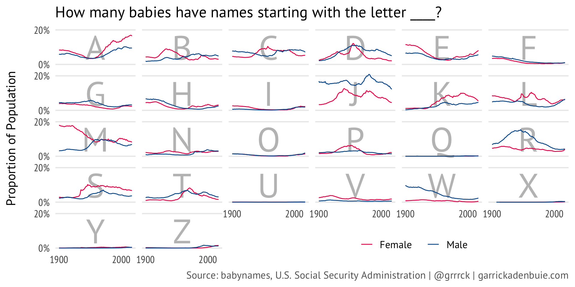
I somewhat like these plots more than their animated versions. I get the sense that I’m seeing a fuller picture (or more easy-to-compare picture) of the overall trends in starting and ending letters of baby names.
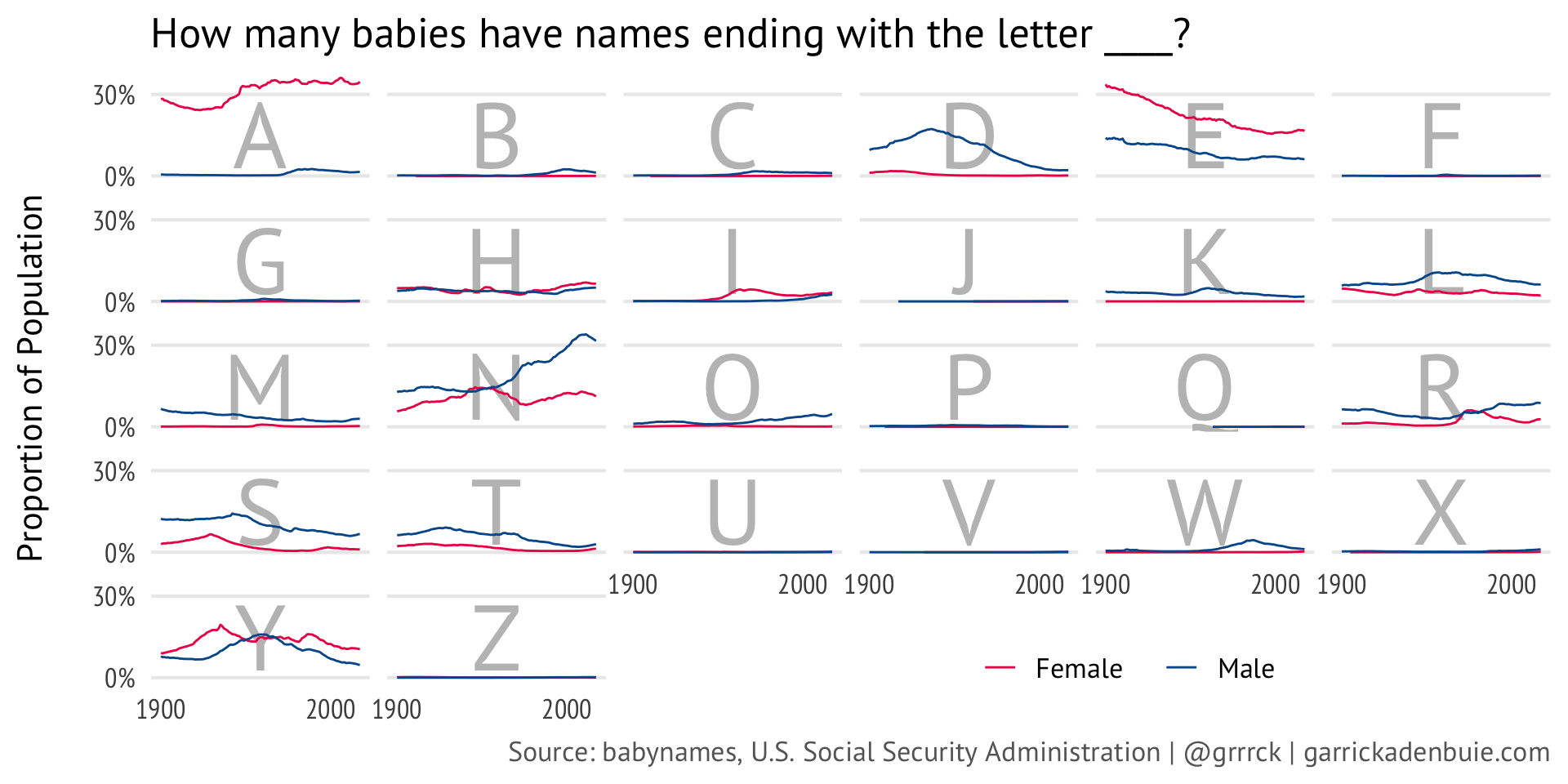
Here’s the code to produce the static image of the trends in the last letter of baby names.
babynames_first_last %>%
  filter(year >= 1900) %>%
  mutate(sex = recode(sex, M = "Male", F = "Female")) %>%
  group_by(year, sex, last_letter) %>%
  summarize(prop = sum(prop)) %>%
  ungroup() %>%
  mutate(last_letter = toupper(last_letter)) %>%
  ggplot() +
  aes(year, prop) +
  geom_text(
    data = tibble(
      last_letter = LETTERS,
      x = 1900+117/2,
      prop = 0
    ),
    aes(label = last_letter, x = x),
    size = rel(15),
    vjust = -0.12,
    color = "grey75",
    family = "PT Sans"
  ) +
  geom_line(aes(color = sex)) +
  facet_wrap(~ last_letter) +
  scale_y_continuous(
    labels = scales::percent_format(5),
    breaks = c(0, 0.3)
  ) +
  scale_x_continuous(breaks = c(1900, 2000)) +
  scale_color_manual(values = sex_colors) +
  labs(
    x = NULL,
    y = "Proportion of Population",
    title = "How many babies have names ending with the letter ____?",
    caption = caption_text,
    color = NULL
  ) +
  base_theme +
  theme(
    strip.text = element_blank(),
    axis.text.x = element_text(face = "plain"),
    legend.position = c(0.7, 0.025),
    panel.grid.minor.y = element_blank()
  )
And here is the code to produce the plot of trends in the first letter of baby names.
babynames_first_last %>%
  filter(year >= 1900) %>%
  mutate(sex = recode(sex, M = "Male", F = "Female")) %>%
  group_by(year, sex, first_letter) %>%
  summarize(prop = sum(prop)) %>%
  ungroup() %>%
  mutate(first_letter = toupper(first_letter)) %>%
  ggplot() +
  aes(year, prop) +
  geom_text(
    data = tibble(
      first_letter = LETTERS,
      x = 1900+117/2,
      prop = 0
    ),
    aes(label = first_letter, x = x),
    size = rel(15),
    vjust = -0.2,
    color = "grey75",
    family = "PT Sans"
  ) +
  geom_line(aes(color = sex)) +
  facet_wrap(~ first_letter) +
  scale_y_continuous(
    labels = scales::percent_format(5),
    breaks = c(0, 0.2)
  ) +
  scale_x_continuous(breaks = c(1900, 2000)) +
  scale_color_manual(values = sex_colors) +
  labs(
    x = NULL,
    y = "Proportion of Population",
    title = "How many babies have names starting with the letter ____?",
    caption = caption_text,
    color = NULL
  ) +
  base_theme +
  theme(
    strip.text = element_blank(),
    axis.text.x = element_text(face = "plain"),
    legend.position = c(0.7, 0.025),
    panel.grid.minor.y = element_blank()
  )
If you made it this far, thanks for reading! I’d love to hear your opinion on these plots, or see your own versions – animated or not! Just drop me a line on Twitter at @grrrck.