The Redacted, Text-Extracted Mueller Report

Earlier today, the redacted Mueller report was released to the public. Only about 12% of the report is redacted, but 100% of it is inside what’s essentially a scanned PDF.

There are many people interested in taking a deeper look at the report, whether within the U.S. government, as citizens, or as data scientists.

Rather than disect the report and its political implications, I’m going to use open-source tools to extract the text from the report. I’m also going to take advantage of the opportunity to use a new R package I’ve been wanting to try, ggpage by Emil Hvitfeldt to visualize the report’s pages and highlight the most-often referenced people in the report.

Extracting the report text with pdftools

I used the pdftools package by ROpenSci to extract the text from the document, using the report posted by @dataeditor of the Washington Post, available here. Extracting the text was as simple as downloading the PDF and running pdftools::pdf_text(). I added page and line numbers to the extracted text and stored the result as a CSV that you can download from the GitHub repository.

library(tidyverse)
library(pdftools)

# Download report from link above
mueller_report_txt <- pdf_text("Redacted-Mueller-Report.pdf")

mueller_report <- tibble(
  page = 1:length(mueller_report_txt),
  text = mueller_report_txt
) %>%
  separate_rows(text, sep = "\n") %>%
  group_by(page) %>%
  mutate(line = row_number()) %>%
  ungroup() %>%
  select(page, line, text)

write_csv(mueller_report, "mueller_report.csv")

Grab the code and resulting data from gadenbuie/mueller-report on GitHub.

Visualizing the report pages with ggpage

The LA Times published an widely-shared piece visualizing each of the pages of the Mueller report, and Nathan Yau of Flowing Data shows how to create this image using pdftools::pdf_convert().

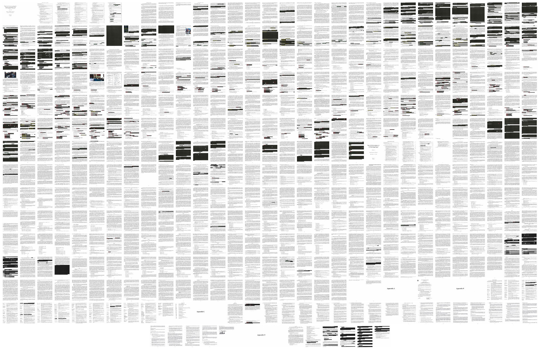
Recently, Emil Hvitfeldt released ggpage, a package that lets you create a page-layout visualization using ggplot2. While the package uses the text content of the document only — so the visualized text layout doesn’t completely match the layout of the original document — it does allow you to highlight text elements, like mentions of any of the recurring cast of characters in Stupid Watergate.

The first step is to load the text version of the Mueller report. You can see from the first few lines of the data that the OCR really struggled with the header that appears at the top of each page and has been crossed out with a single line. (The redacted text is less confusing to the OCR because it’s rendered in solid black and generally results in blank space.)

library(tidyverse)
library(ggpage)

mueller_report_csv <- "https://raw.githubusercontent.com/gadenbuie/mueller-report/ab74012b0532ffa34f3a45196d2b28004e11b9c2/mueller_report.csv"

mueller_report <- read_csv(mueller_report_csv)

mueller_report

# A tibble: 19,195 × 3
    page  line text                                             
   <dbl> <dbl> <chr>                                            
 1     1     1 "U.S. Department of Justice"                     
 2     1     2 "AttarAe:,c\\\\'erlc Predtiet // Mtt; CeA1:ttiA" 
 3     1     3 "Ma1:ertalPrn1:eetedUAder Fed. R. Crhtt. P. 6(e)"
 4     1     4 "Report On The Investigation Into"               
 5     1     5 "Russian InterferenceIn The"                     
 6     1     6 "2016 PresidentialElection"                      
 7     1     7 "Volume I of II"                                 
 8     1     8 "Special Counsel Robert S. Mueller, III"         
 9     1     9 "Submitted Pursuant to 28 C.F.R. § 600.8(c)"     
10     1    10 "Washington, D.C."                               
# … with 19,185 more rows

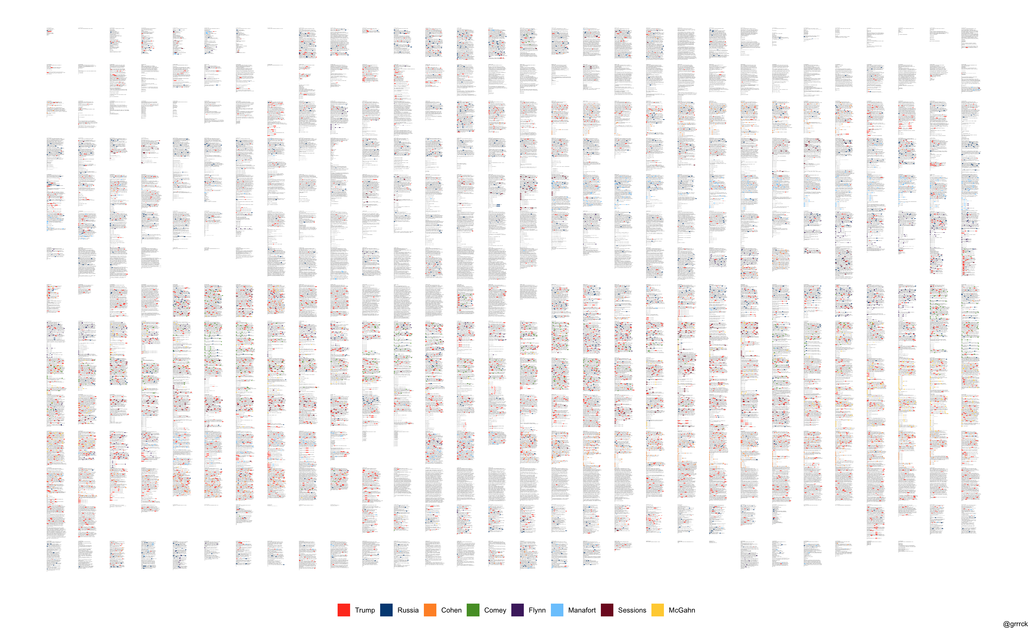
The core of the next step is to pass the mueller_report to ggpage::ggpage_build(). Before doing that, though, I pad each page to make sure they have the same number of lines. The ggpage_build() function tokenizes the text into individual words, so I then use str_detect() to find mentions of the key players.

mueller_pages <-
  mueller_report %>%
  # pad pages with fewer lines than expected
  complete(
    page,
    line = 1:max(mueller_report$line),
    fill = list(text = "")
  ) %>%
  # Pre-process for {ggpage}
  ggpage_build(
    ncol = 30,
    bycol = FALSE,
    page.col = "page",
    wtl = FALSE,
    x_space_pages = 10,
    y_space_pages = 100
  ) %>%
  mutate(
    color = case_when(
      str_detect(word, "trump|president") ~ "Trump",
      str_detect(word, "russia")     ~ "Russia",
      str_detect(word, "cohen")      ~ "Cohen",
      str_detect(word, "co(m|rn)ey") ~ "Comey",
      str_detect(word, "flynn")      ~ "Flynn",
      str_detect(word, "manafort")   ~ "Manafort",
      str_detect(word, "sessions")   ~ "Sessions",
      str_detect(word, "mcgahn")     ~ "McGahn",
      TRUE ~ "normal"
    ),
    color = factor(color, c(
      "Trump", "Russia", "Cohen", "Comey",
      "Flynn", "Manafort", "Sessions", "McGahn", "normal"
    ))
  )

mueller_pages

# A tibble: 207,165 × 9
   word        page  line  xmin  xmax  ymin  ymax index_line color 
   <chr>      <dbl> <dbl> <dbl> <dbl> <dbl> <dbl> <chr>      <fct> 
 1 u.s            1     1   175   172  -204  -207 1-1        normal
 2 department     1     1   186   176  -204  -207 1-1        normal
 3 of             1     1   189   187  -204  -207 1-1        normal
 4 justice        1     1   197   190  -204  -207 1-1        normal
 5 washington     1    10   182   172  -240  -243 1-10       normal
 6 d.c            1    10   186   183  -240  -243 1-10       normal
 7 march          1    11   177   172  -244  -247 1-11       normal
 8 2019           1    11   182   178  -244  -247 1-11       normal
 9 attarae        1     2   179   172  -208  -211 1-2        normal
10 c              1     2   181   180  -208  -211 1-2        normal
# … with 207,155 more rows

The following bit of code sets up the color palette, which is derived from the Libre Office Calc theme provided by ggthemes.

# manually assigned colors from ggthemes::pal_calc()
colors <- rep("", length(levels(mueller_pages$color)))
names(colors) <- levels(mueller_pages$color)
colors["Trump"]    <- "#FF4023"
colors["Russia"]   <- "#004983"
colors["Cohen"]    <- "#FF922E"
colors["Comey"]    <- "#559B30"
colors["Flynn"]    <- "#4D276D"
colors["Manafort"] <- "#7BCAFD"
colors["Sessions"] <- "#7F1327"
colors["McGahn"]   <- "#FFD040"
colors["normal"]   <- "#d0d0d0"

Finally, ggpage_plot() from ggpage creates the ggplot2 page layout, and adding the fill aesthetic using the manual color scale defined above adds color highlights for mentions of Trump, Russia, and others.

ggpage_plot(mueller_pages) +
  aes(fill = color) +
  scale_fill_manual(
    values = colors,
    breaks = setdiff(names(colors), "normal")
  ) +
  labs(fill = NULL, caption = "@grrrck") +
  guides(fill = guide_legend(nrow = 1)) +
  theme(legend.position = "bottom")

Click the image to expand.

---

If you use the data for an interesting visualization or analysis, please let me know on Twitter!

Source: LA Times