🤹 tidyexplain

Project

Animations of tidyverse verbs using R, the tidyverse, and gganimate.

Published

August 27, 2018

Source

Tidy Animated Verbs

Follow @gadenbuie Star Fork

Mutating Joins — inner_join(), left_join(), right_join(), full_join()
Filtering Joins — semi_join(), anti_join()
Set Operations — union(), union_all(), intersect(), setdiff()
Tidy Data — pivot_wider() and pivot_longer(), spread() and gather()
Learn more about

Background

Usage

Please feel free to use these images for teaching or learning about action verbs from the tidyverse. You can directly download the original animations or static images in svg or png formats, or you can use the scripts to recreate the images locally.

Currently, the animations cover the dplyr two-table verbs and I’d like to expand the animations to include more verbs from the tidyverse. Suggestions are welcome!

Relational Data

The Relational Data chapter of the R for Data Science book by Garrett Grolemund and Hadley Wickham is an excellent resource for learning more about relational data.

The dplyr two-table verbs vignette and Jenny Bryan’s Cheatsheet for dplyr join functions are also great resources.

gganimate

The animations were made possible by the newly re-written gganimate package by Thomas Lin Pedersen (original by Dave Robinson). The package readme provides an excellent (and quick) introduction to gganimate.

Dynamic Animations

Thanks to an initial push by David Zimmermann, we have begun work towards functions that generate dynamic animations from users’ actual data. Please visit the pkg branch of the tidyexplain repository for more information (or to contribute!).

Mutating Joins

A mutating join allows you to combine variables from two tables. It first matches observations by their keys, then copies across variables from one table to the other.
R for Data Science: Mutating joins

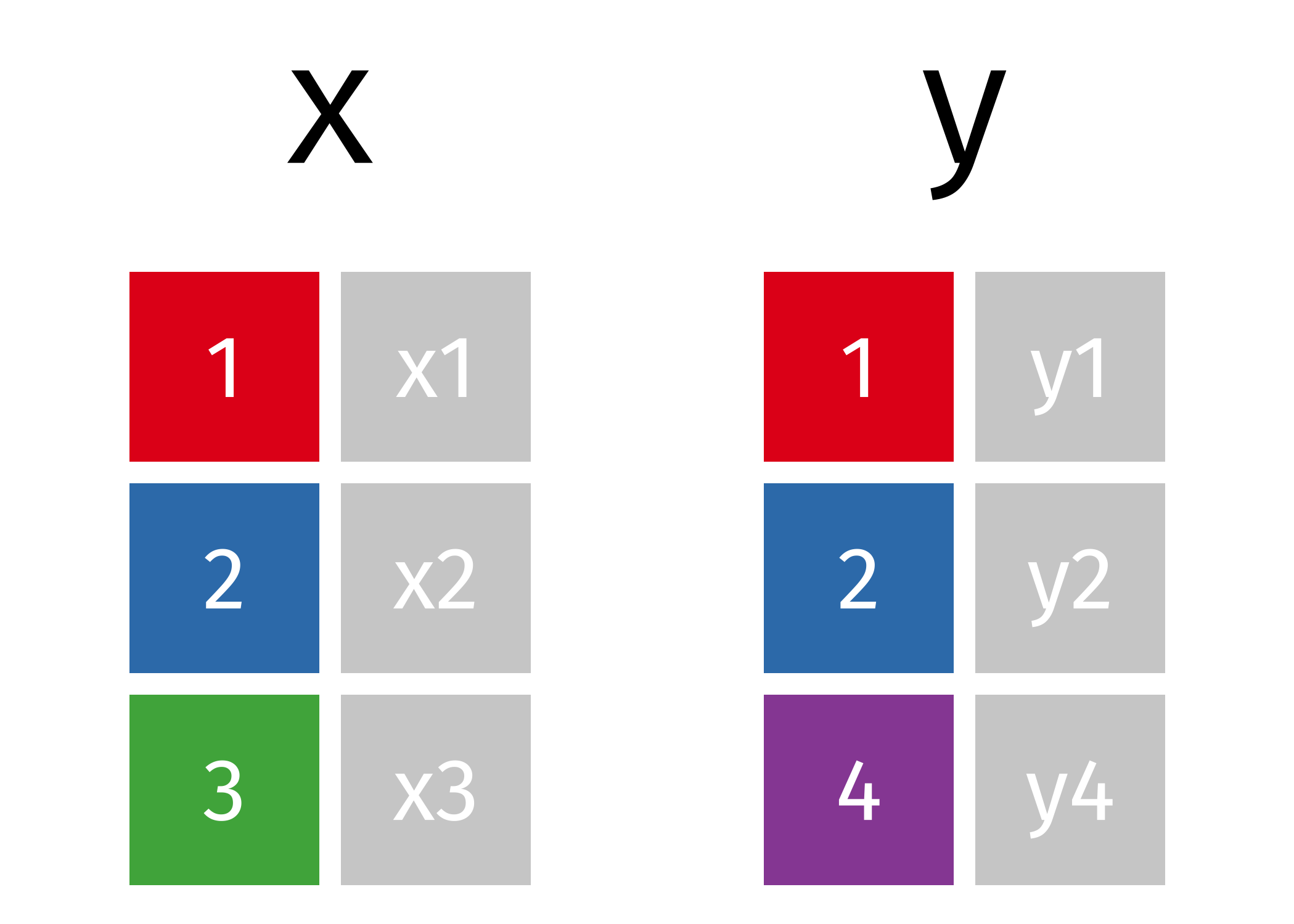
x
#> # A tibble: 3 × 2
#>      id x    
#>   <int> <chr>
#> 1     1 x1   
#> 2     2 x2   
#> 3     3 x3
y
#> # A tibble: 3 × 2
#>      id y    
#>   <int> <chr>
#> 1     1 y1   
#> 2     2 y2   
#> 3     4 y4

Inner Join

All rows from x where there are matching values in y, and all columns from x and y.

inner_join(x, y, by = "id")
#> # A tibble: 2 × 3
#>      id x     y    
#>   <int> <chr> <chr>
#> 1     1 x1    y1   
#> 2     2 x2    y2

Left Join

All rows from x, and all columns from x and y. Rows in x with no match in y will have NA values in the new columns.

left_join(x, y, by = "id")
#> # A tibble: 3 × 3
#>      id x     y    
#>   <int> <chr> <chr>
#> 1     1 x1    y1   
#> 2     2 x2    y2   
#> 3     3 x3    <NA>

Left Join (Extra Rows in y)

… If there are multiple matches between x and y, all combinations of the matches are returned.

y_extra # has multiple rows with the key from `x`
#> # A tibble: 4 × 2
#>      id y    
#>   <dbl> <chr>
#> 1     1 y1   
#> 2     2 y2   
#> 3     4 y4   
#> 4     2 y5
left_join(x, y_extra, by = "id")
#> # A tibble: 4 × 3
#>      id x     y    
#>   <dbl> <chr> <chr>
#> 1     1 x1    y1   
#> 2     2 x2    y2   
#> 3     2 x2    y5   
#> 4     3 x3    <NA>

Right Join

All rows from y, and all columns from x and y. Rows in y with no match in x will have NA values in the new columns.

right_join(x, y, by = "id")
#> # A tibble: 3 × 3
#>      id x     y    
#>   <int> <chr> <chr>
#> 1     1 x1    y1   
#> 2     2 x2    y2   
#> 3     4 <NA>  y4

Full Join

All rows and all columns from both x and y. Where there are not matching values, returns NA for the one missing.

full_join(x, y, by = "id")
#> # A tibble: 4 × 3
#>      id x     y    
#>   <int> <chr> <chr>
#> 1     1 x1    y1   
#> 2     2 x2    y2   
#> 3     3 x3    <NA> 
#> 4     4 <NA>  y4

Filtering Joins

Filtering joins match observations in the same way as mutating joins, but affect the observations, not the variables. … Semi-joins are useful for matching filtered summary tables back to the original rows. … Anti-joins are useful for diagnosing join mismatches.
R for Data Science: Filtering Joins

Semi Join

All rows from x where there are matching values in y, keeping just columns from x.

semi_join(x, y, by = "id")
#> # A tibble: 2 × 2
#>      id x    
#>   <int> <chr>
#> 1     1 x1   
#> 2     2 x2

Anti Join

All rows from x where there are not matching values in y, keeping just columns from x.

anti_join(x, y, by = "id")
#> # A tibble: 1 × 2
#>      id x    
#>   <int> <chr>
#> 1     3 x3

Set Operations

Set operations are occasionally useful when you want to break a single complex filter into simpler pieces. All these operations work with a complete row, comparing the values of every variable. These expect the x and y inputs to have the same variables, and treat the observations like sets.
R for Data Science: Set operations

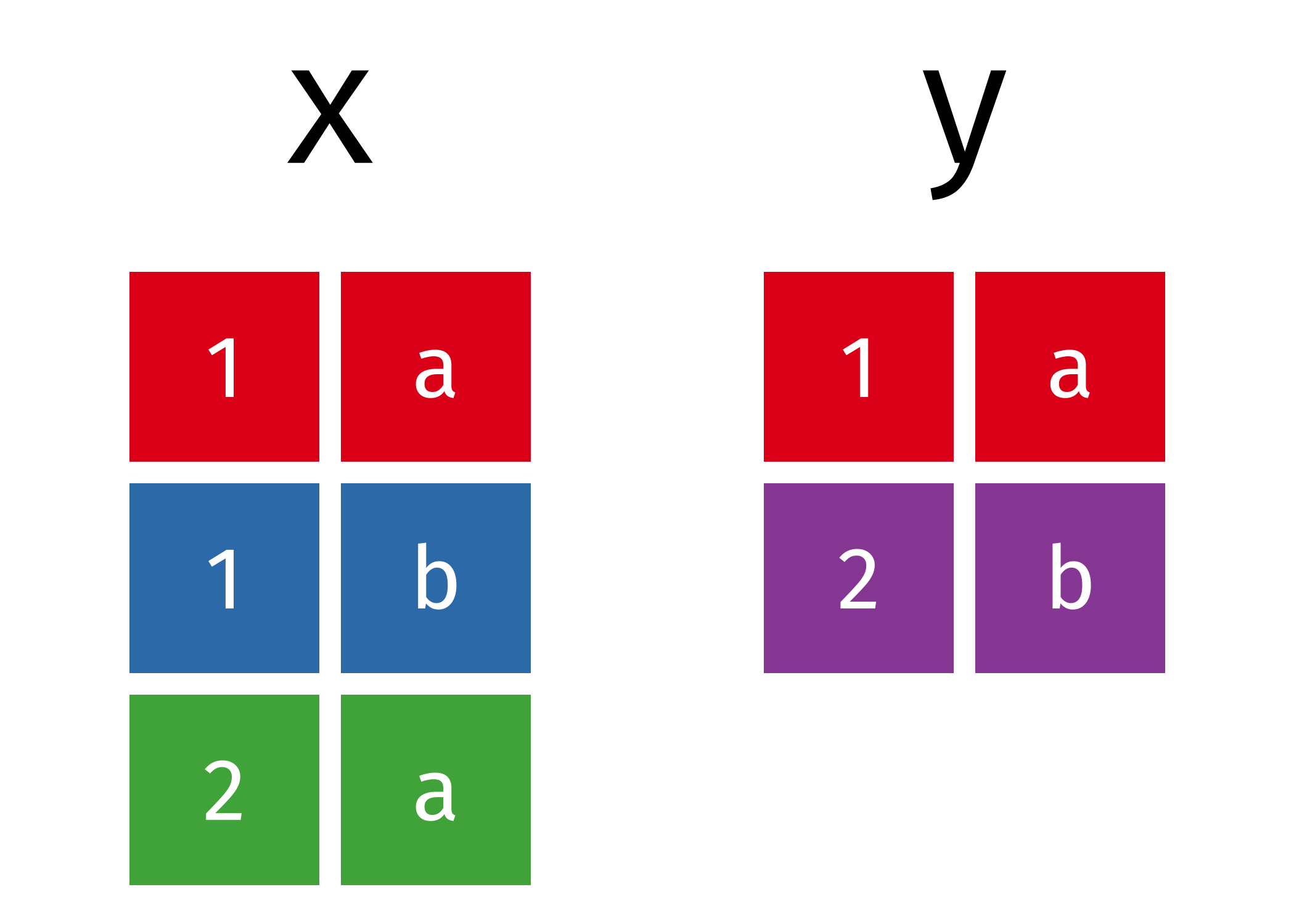
x
#> # A tibble: 3 × 2
#>   x     y    
#>   <chr> <chr>
#> 1 1     a    
#> 2 1     b    
#> 3 2     a
y 
#> # A tibble: 2 × 2
#>   x     y    
#>   <chr> <chr>
#> 1 1     a    
#> 2 2     b

Union

All unique rows from x and y.

union(x, y)
#> # A tibble: 4 × 2
#>   x     y    
#>   <chr> <chr>
#> 1 1     a    
#> 2 1     b    
#> 3 2     a    
#> 4 2     b

union(y, x)
#> # A tibble: 4 × 2
#>   x     y    
#>   <chr> <chr>
#> 1 1     a    
#> 2 2     b    
#> 3 1     b    
#> 4 2     a

Union All

All rows from x and y, keeping duplicates.

union_all(x, y)
#> # A tibble: 5 × 2
#>   x     y    
#>   <chr> <chr>
#> 1 1     a    
#> 2 1     b    
#> 3 2     a    
#> 4 1     a    
#> 5 2     b

Intersection

Common rows in both x and y, keeping just unique rows.

intersect(x, y)
#> # A tibble: 1 × 2
#>   x     y    
#>   <chr> <chr>
#> 1 1     a

Set Difference

All rows from x which are not also rows in y, keeping just unique rows.

setdiff(x, y)
#> # A tibble: 2 × 2
#>   x     y    
#>   <chr> <chr>
#> 1 1     b    
#> 2 2     a

setdiff(y, x)
#> # A tibble: 1 × 2
#>   x     y    
#>   <chr> <chr>
#> 1 2     b

Tidy Data

Tidy data follows the following three rules:

Each variable has its own column.
Each observation has its own row.
Each value has its own cell.

Many of the tools in the tidyverse expect data to be formatted as a tidy dataset and the tidyr package provides functions to help you organize your data into tidy data.

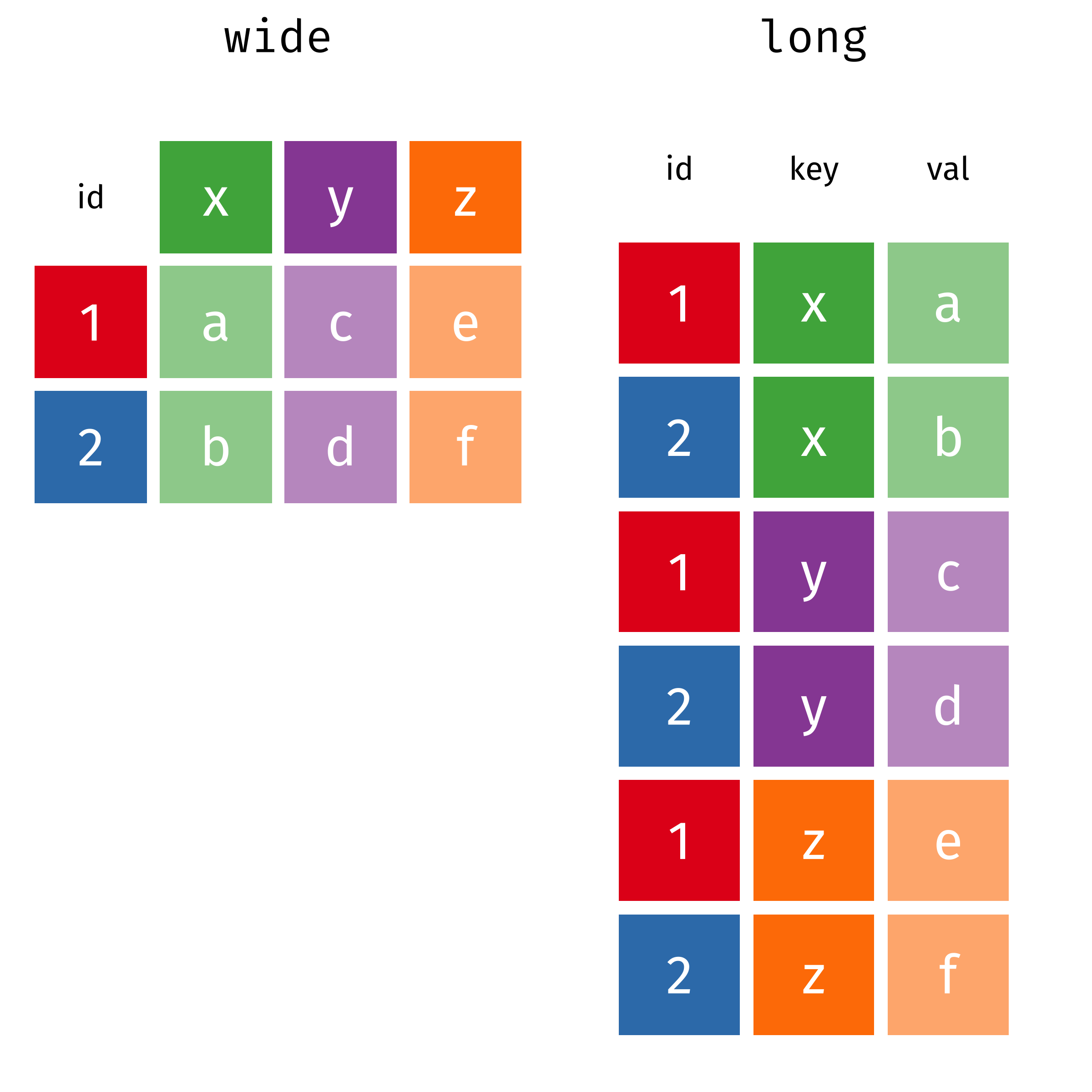
wide
#> # A tibble: 2 × 4
#>      id x     y     z    
#>   <int> <chr> <chr> <chr>
#> 1     1 a     c     e    
#> 2     2 b     d     f
long
#> # A tibble: 6 × 3
#>      id key   val  
#>   <int> <chr> <chr>
#> 1     1 x     a    
#> 2     2 x     b    
#> 3     1 y     c    
#> 4     2 y     d    
#> 5     1 z     e    
#> 6     2 z     f

Pivot Wider and Longer

pivot_wider() and pivot_longer() were introduced in tidyr version 1.0 (released in September 2019). They provide a more consistent and more powerful approach to changing the fundamental shape of the data and are “modern alternatives to spread() and gather().

Here we show the very basic mechanics of pivoting, but there’s much more that the pivot functions can do. You can learn more about them in the Pivoting vignette in tidyr.

pivot_wider(data, names_from = key, values_from = val)

pivot_wider() “widens” data, increasing the number of columns and decreasing the number of rows.

pivot_longer(data, cols = x:y, names_to = "key", values_to = "val")

pivot_longer() “lengthens” data, increasing the number of rows and decreasing the number of columns.

Spread and Gather

spread(data, key, value)

Spread a key-value pair across multiple columns. Use it when an a column contains observations from multiple variables.

gather(data, key = "key", value = "value", ...)

Gather takes multiple columns and collapses into key-value pairs, duplicating all other columns as needed. You use gather() when you notice that your column names are not names of variables, but values of a variable.

gather(wide, key, val, x:z)
#> # A tibble: 6 × 3
#>      id key   val  
#>   <int> <chr> <chr>
#> 1     1 x     a    
#> 2     2 x     b    
#> 3     1 y     c    
#> 4     2 y     d    
#> 5     1 z     e    
#> 6     2 z     f
spread(long, key, val)
#> # A tibble: 2 × 4
#>      id x     y     z    
#>   <int> <chr> <chr> <chr>
#> 1     1 a     c     e    
#> 2     2 b     d     f